Storage and Retrieval

Two families of storage engines:

• log-structured storage
• page-oriented storage

Data Structures That Power Your Database

• Logs - append-only data file
• Indexes - additional structures to help increase performance by shortening the look up path

Indexes

Hash Indexes

KV data. Indexes based on KV data.

Reducing footprint:

• Compaction - break the log into segments of a given epoch size, older segments can be compacted by throwing away duplicates keys in log and keeping the most recent update for each key
  • Potentially idea referenced from LFS Segment Cleaning mechanism

Hash Index Implementation Problems

• File format - Simplest and smallest is length followed by string of bytes, length value acting as delimiter. Increases complexity for parsing
• Deleting records - Deleting key values requires a special deletion record to data file (tombstone). The record marks the data to discard previous values for key.
• Crash recovery - Requires backup of in-memory data to disk
• Partially written records - Use checksums to ignore corrupted parts of the log
• Concurrency control - One writer thread. Data file segments are append-only and otherwise immutable, allowing for multiple reader threads

Hash table index has limitations:

• Hash table must fit in memory, difficult to maintain performance with database stored partially on disk.
• Range queries are not efficient. Hash indexes have to scan over all keys in hash map

SSTables and LSM-Trees

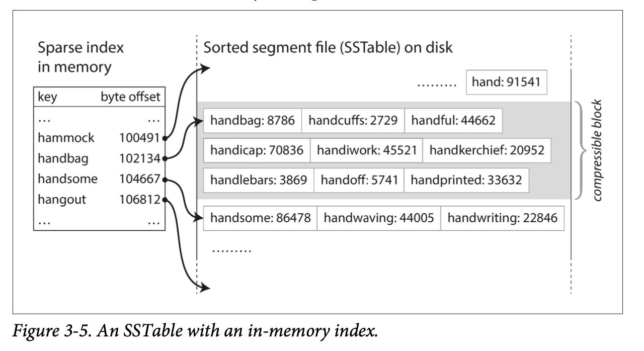
SSTable or Sorted String Table - the requirement is that KV pairs are sorted by key SSTables advantages over log segments with hash indexes:

1. Merging segments is simple and efficient, even if files are bigger than available memory. Files segments are sorted.
2. No longer need to keep an index of all keys in memory. Keys can be sparse and due to sort, the target key that’s not defined in memory can be deduced to be in-between keys.
3. Since read request to scan over several KV pairs in range anyways. Can group records into a block and send the block over to disk to reduce I/O
   • Able to batch read request within a key range due to locality

LSM-tree - Log-structured Merge Tree; merging and compacting sorted files in the same fashion as SSTables

• Since disk writes are sequential, LSM-tree can support high write throughput
• variable-sized
• Implementation below

Constructing and maintaining SSTables

Memtable - in-memory tree

Implementation Details

• On write request, inserted into a balanced memtable
• When the table exceeds memory threshold write out to disk as a SSTable file
• On read request, search memtable, then disk segment, and then the next-older segment.
• From time to time, run merging and compaction process in the background to combine segment files and discard overwritten and deleted files

B-Trees

Most widely used indexing structure.

Uses KV pairs sorted by keys (like SSTables). The difference is that B-trees break the DB down to fixed-sized blocks.

• Efficient value lookups and rage queries

Def: An ordered search tree where each node keeps a sorted list of keys.

Reliability: B-Tree implementaitons includes an addition data structure on disk called a write-ahead log or WAL or redo log. This is an append-only file to which every B-tree modification must be written before it can be applied to the pages of the tree itself.

B-Trees vs LSM-Trees

B-Trees	LSM-Trees
Fixed sized blocks	Variable sized blocks
Faster for reads, fixed size blocks typically are smaller than LSM-tree sized blocks, more fine grained search	Faster for writes, no need to balance tree on every write. Reads slower because of potential duplicates prior to compaction
Has to write every piece of data twice (once to WAL, sec. to tree)	Rewrite data multiple times due to compaction and merging of SSTables, write amplification
”Balances on write"	"Compacts and merges on cron”, may affect performance
fragmentation due to fixed sized	increased disk utilization
Each key exists exactly in one place in the index	may have multiple copies of the same key in different segments

Other Indexing Structures

Primary and Secondary indexes

• Create indexes within indexes

Storing values within the index

Values can be two different types: the actual row or the reference to the row stored elsewhere (heap file)

Heap file - stores data in no particular order, avoids deduplicating data when multiple secondary indexes are present. Each index references a location in heap file.

• Extra hop from index to heap file can be too much of a performance penalty for reads
• Can have better utilization of storage

Clustered index - storing the indexed row directly within an index. Secondary indexes refer to primary key.

Multi-column indexes

For querying multiple columns of a table.

Most common type of multi-column index is called a concatenated index which combines several fields into on key by appending one column to another.

• Eg. (lastname, firstname) to phone number

Full-text search and fuzzy indexes

Full-text search indexes - indexes for searching for relevance in query, using keyword search, stemming/tokenization, synonyms, and other properties. Fuzzy indexes - indexes for fuzzy search

Lucene uses a SSTable-like structure for its term dictionary.

• This in-memory index is like a finite state automation over the characters in the keys.
• like trie

Levenshtein automaton - number in which x can be transformed into w by at most n single-character insertions, deletions, and substitutions.

• used in spelling

In-Memory Databases

As RAM becomes cheaper, it becomes more feasible to keep them entirely in memory and potentially distributed.

Relational in-memory: VoltDB, MemSQL, and Oracle TimesTen

In-memory database can hold datasets larger than available memory, but using an anti-caching approach

• Anti-caching - evicts LRU data from memory to disk and pulls it in when it’s accessed again.

RIP NVM tech lmao

Transaction Processing or Analytics?

Transaction - group of reads and writes that form a logical unit

Transaction doesn’t necessarily need to have ACID properties. Transaction processing just means to allow clients to make low-latency reads and writes rather than batch processing jobs (runs periodically)

Online transaction processing (OLTP) - access pattern for when records are inserted or updated based on the user’s input

Data analytics bring along other different access patterns.

• Analytic queries needs to scan over a huge number of records, only reading a few columns per record, and calculates aggregate stats
• These patterns are called Online analytic processing (OLAP)

OLTP vs OLAP

Property	Property Transaction processing systems (OLTP)	Analytic systems (OLAP)
Main read pattern	Small number of records per query, fetched by key	Aggregate over large number of records
Main write pattern	Random-access, low-latency writes from user input	Bulk import (ETL) or event stream
Primarily used by	End user/customer, via web application	Internal analyst, for decision support
What data represents	Latest state of data (current point in time)	History of events that happened over time
Dataset size	Gigabytes to terabytes	Terabytes to petabytes
Query properties	Typically more volume of queries	Queries are typically more demanding

Data Warehousing

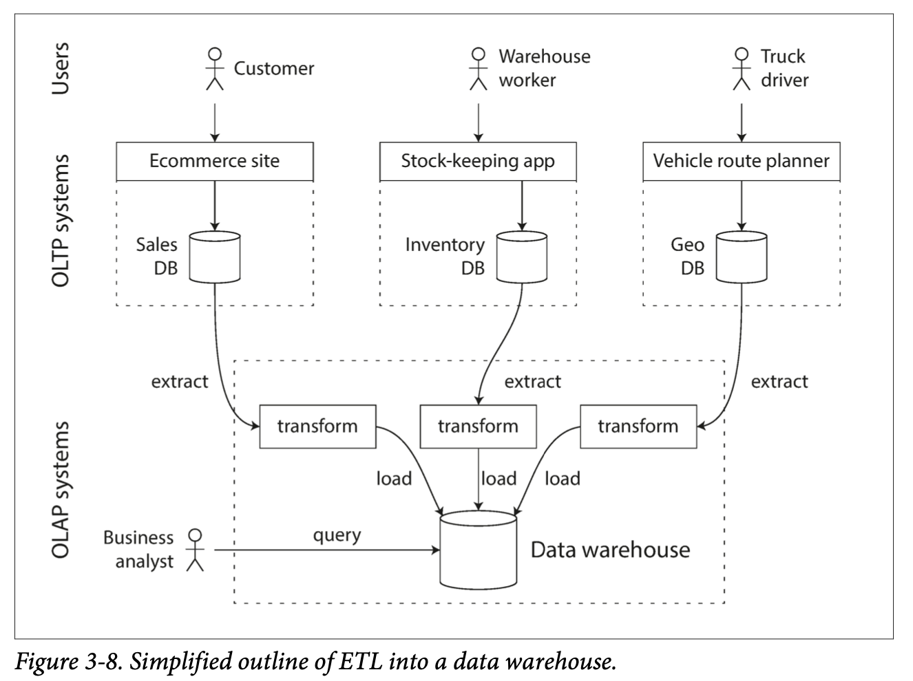
Data warehouse - separate databases used to store analytics and reporting

• Contains a read-only copy of the data in various OLTP systems in the company.
• Data is extracted from OLTP databases and transformed into an analysis-friendly schema, cleaned up, and then loaded into the data warehouse. Extract-Transform-Load (ETL)

Stars and Snowflakes: Schemas for Analytics

Transaction processing has a wide range of different data models, depending on the needs of the application

On the other hand, in analytics, there is much less diversity of data models. Many data warehouses use star schema or dimensional modeling

Star Schema / Dimensional Modeling

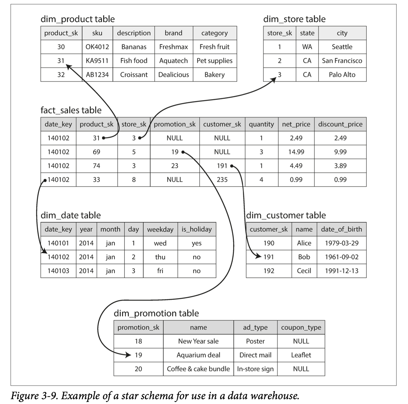
• Center of the schema is a fact table, each row of the fact table represents an event that occurred at a particular time.
  • If we were analyzing website traffic rather than retail sales, each row might represent a page view or click by user.
  • Allows for the maximum flexibility of analysis later, but can be quite large
• The fact table has columns that are foreign key references to dimension tables. Each row in the dimension tables represents who, what, where, when, how, and why of the event.

Snowflake Schema, variation of star

Dimensions are further broken down into subdimensions which makes snowflake schemas more normalized than star schemas. But star schemas are often preferred because they are simpler for analysts to work with.

Column-Oriented Storage

Fact tables are often over 100 columns wide, but a typical query only accesses 4 or 5 of them at once.

Typically OLTP DBs storage is laid out in row-oriented fashion. We can have indexes on foreign keys. But for a row-oriented storage engine, it still needs to load all those rows with all their column data from disk into memory, parse them, and filter. This includes additional dimensions from the original dimensional table.

Use column-oriented storage instead. The idea is don’t store all the values form one row together, but store the values from each column together instead. If each column is stored in a separate file, a query only needs to read and parse those columns that are used in that query.

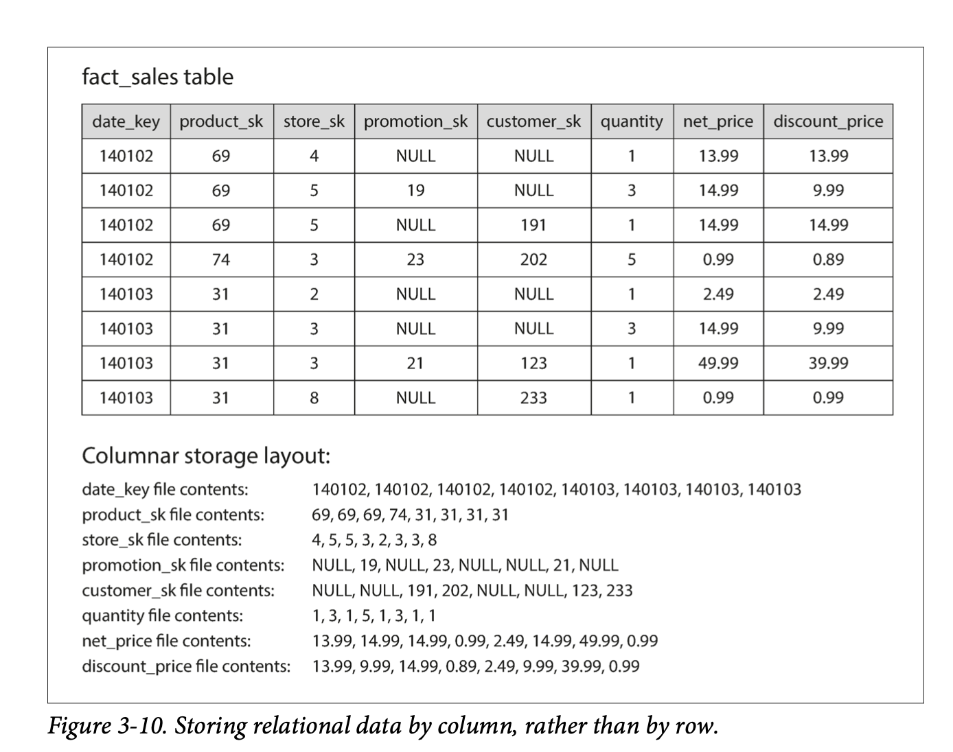
• Building a row is taking the index of each column needed.

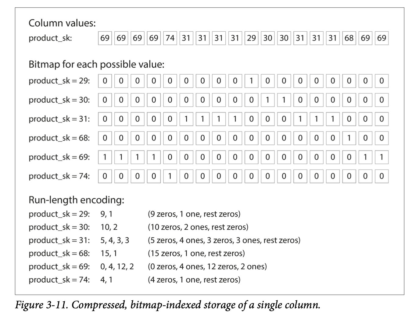
Column Compression

Bitmap encoding

Example query:

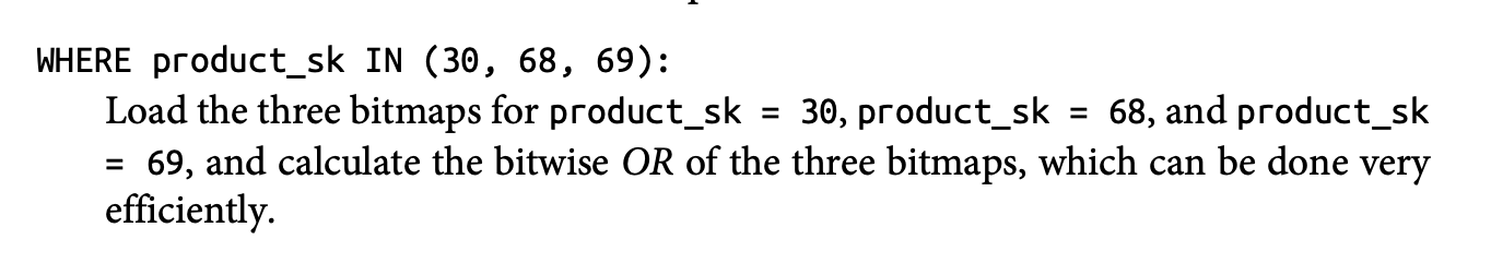
• Finds product_sk either in 30, 68, 69 Example query 2: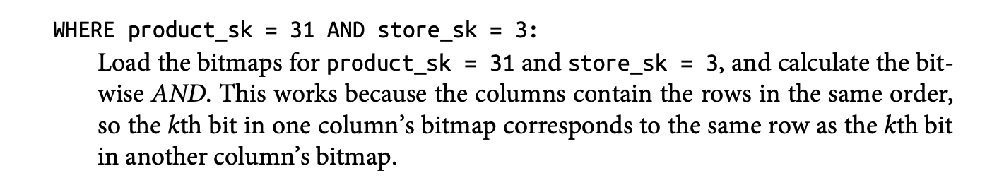

Memory Bandwidth and Vectorized Processing

For data warehouse queries that need to scan over millions of rows, a big bottleneck is the bandwidth for getting data from disk into memory

• Also efficiently using bandwidth from main memory into the CPU cache, avoiding branch mispredicitons and bubbles in CPU instruction processing pipeline.

Vectorized processing - use bitwise AND and OR to operate on chunks of compressed column data directly. See above queries.

• Compressed column data also allows more rows to fit into limited cache space.

Sort Order in Column Storage

All columns need to be sorted at once or an entire row at a time to preserve data cohesion.

Pros:

• Sorting helps with compression of columns; eg. run-length encoding for common values
• Increased search performance due to sorted ranges

Idea: several different sort orders Different queries benefit from different sort orders, so why not store the same data but sorted in several different ways?

Writing to Column-Oriented Storage

Due to compression and sorting in column-oriented storage, writes are more difficult.

Update-in-place (B-trees) is not possible with compressed columns. You would have to rewrite all the column files, due to column index potentially breaking contagious values. (think Run-length encoding and a bit is changed in the middle of a contagious region)

What we can use is logs (LSM-tree), writes first go to an in-memory store, where they are added to a sorted structure and prepared for writing to disk.

• Merge with column files on disk and written to new files in bulk maintains rows.

Aggregation: Data Cubes and Materialized Views

Materialized aggregates - caching aggregate functions

One way to create such a cache is a materialized view.

• In relational data model, a standard (virtual) view is a table-like object whose contents are the results of some query.
• The difference here, is the materialized view is an actual copy of the query results, whereas the virtual view is a shortcut for writing queries.

Issue is that materialized views deal with cache coherency issues and maintaining the updated state is expensive.

• Which is why it’s not used in OLTP databases.
• In read-heavy data warehouses, it can make more sense

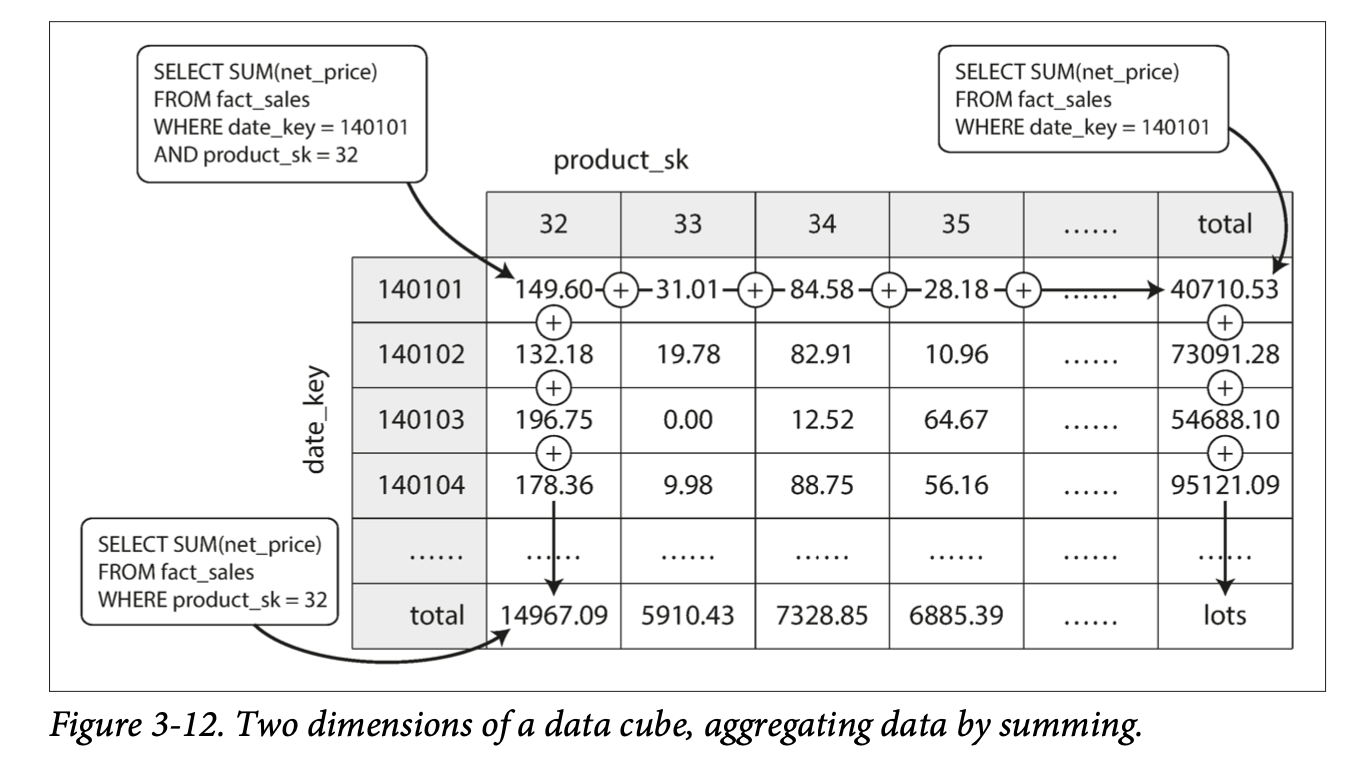
A common case of a materialized view is: data cube or OLAP cube

• Grid of aggregates grouped by different dimensions